― Rachel Carson, author of Silent Spring
The Big Bang Theory
Three minutes after the Big Bang, the Universe temperature had fallen below 1 billion degrees and its diameters had grown to about 100 billion km (60 billion miles). As the Universe continued to expand and cool further, atoms and molecules slowed down and accumulated into nebulae, patchy clouds of gas consisted entirely of the smallest atoms - hydrogen (98%), helium (2%) and traces of lithium, beryllium, and boron.

Protostars were formed when the gravitational pull of nebulae began pulling in its surrounding gases and gradually grew in mass and therefore, density. This grand example of "rich getting richer" meant the denser region of matter compacted into a smaller region with other gases swirling around it resulting a spinning disk-shaped mass of gas called an accretion disc.
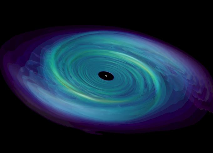
The formation of this disc meant as the centre got denser as the gravitational pull increased resulting in the inward collapse of the surrounding nebula. This kinectic motion of atoms and molecules towards the centre transformed into heat and increased temperature of this "ball". The constant movement of the atoms and molecules inside the ball further increased the temperature till it became hot enough to glow, thus becoming a protostar. As the protostar pulls in more mass, its core becomes dense enough for the temperature to reach about 10 million degrees which sets the stage for fusion reactions (which in a nutshell means formation of heavier elements i.e. hydrogen nuclei join to form helium nuclei). The protostar has now officially become a star.
"We are all made of stardust"
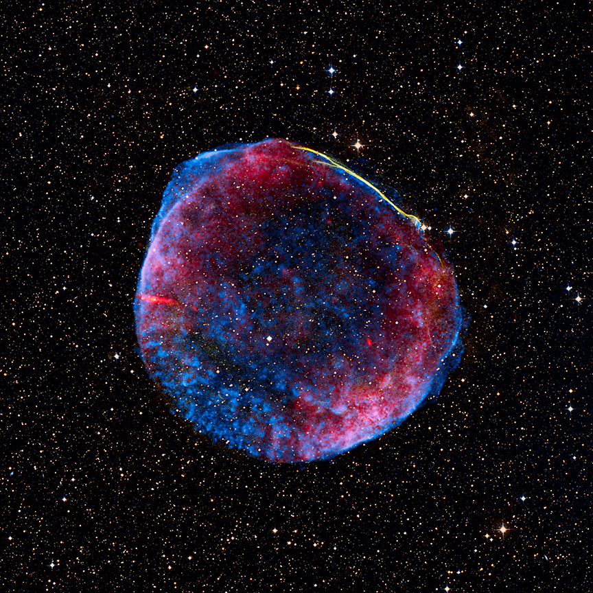
The first-generation stars were huge compared to our Sun (100x Sun's mass). The bigger these stars were, the quicker they burn. Low-mass stars like our Sun burn slowly and will be probably survie for 10 billion years while the high-mass stars survive for only 20 million years. These high-mass stars die by violently exploding into a supernova while smaller stars like our Sun die by releasing a large shell of gas. These atoms which are released back into space go on to form new nebulae or mix back into existing nebulae. The first-generation starts left a legacy of new elements which was used by the next generation of stars. Low-mass stars such as our Sun produce elements upto an atomoic number of 6 (carbon) while high-mass stars produce elements upto to an atomic number of 26 (iron). Larger atoms are formed during a supernova explosion and also in some extremely massive stars. Hence, our Earth and therefore our body, also contains a mix of these elements - basically formed from the exploding stars!
Our Solar System
Our Solar System was formed 4.56 billion years or over 9 billion years after the big bang, making our Sun a third/fourth/fifth generation star (hard to confirm for sure). Since our Solar System was late to this "party", the accretion disc formed around our Sun consisted not just of gas but also "dust" and ice. Such an accretion disc is also called a proto-planetary disc because it contains the raw materials from which planets form. Over time, the center of this disc formed the proto-Sun while the remainder evolved into concentric rings with the warmer inner rings containing higher concentration of dust and the outer rings containing ice. Note that the Sun contains 99.98% of mass in our Solar System and the Jupiter (318 times our Earth's mass) contains 99.5% of all nonsolar mass in our Solar System.

Meteorites
- Jack London
Meteorites are the extra-terresterial materials usually made of iron and could have been formed millions or billions years ago. Most of them could be part of planets or large asteroids in the Asteroid belt (Ceres - largest body in the Asteroid belt was visited March 7!). The rare ones could have been formed at the time of our Solar system and are called Chondrules. It is fascinating we can study materials that were part of our Solar nebula.
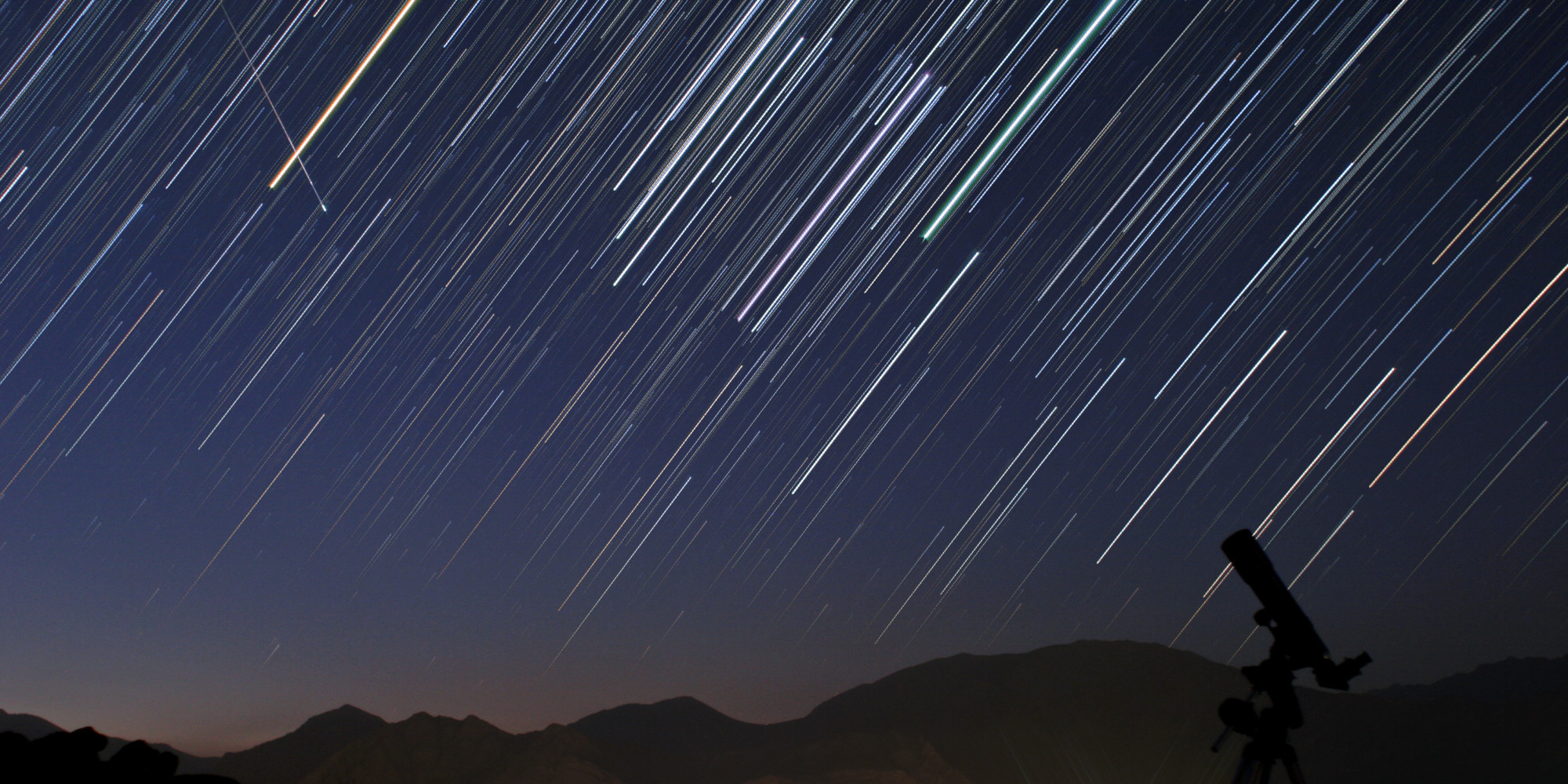
Note that meteorites are different from meteors. Meteor is a scientific name for a shooting star. The heat generated by the friction with our Earth's atmosphere results in a bright, short-lived flame. Meteor showers periodic throughout the year and you can find the list of major showers here .
As most of the meteorites are from the Asteroid belt, it should be noted that the total combined mass of the asteroids in the Asteroid belt is around the mass of our Moon. In addition, astronomers have found about a 1,000 asteroids with diameters greater than 30km. There are supposed to be over 10 million asteriods with diameter less than a km.
Curiosity:
For this project, I would like to explore and learn about the different sizes and types of meteorites. It would also be interesting to check when these meteorites fell on Earth as the dataset claims to have record of every meteorite since 2600 B.C.
Analysis:
We will analyze the meteorite dataset based on the US Meteoritical Society.
First, we import the necessary python libraries and read the our dataset which is in csv format. We want to find out the size of our dataset and also print the first row to take a look at the column headings and data types and values.
import sys,os
import pandas as pd
import numpy as np
import matplotlib
import matplotlib.pyplot as plt
import seaborn as sns

meteorites = pd.read_csv('meteorites.csv') #read our dataset and stores it in "meteorites" variable
print(meteorites.shape) #size of our dataset
meteorites.head(1) #prints first row of our dataset
There are over 34,000 items (row entries) with 15 categories (column entries). Looking at our first row, we see the dataset also provides us with the latitude and longitude coordinates. Let's plot these on our world map!
fig=plt.figure(figsize=(10,5))
plot(meteorites['longitude'], meteorites['latitude'], '.', color = 'lightGreen')

This gives us a nice image and it is not surprising to see the meteorites to map exactly over the continents. Next, let us dive deeper into the dataset. Since one of the things I wanted to explore was the type of meteorites, let's do a quick check on the different types we have.
meteoriteTypes = pd.unique(meteorites['type_of_meteorite'].ravel())
print(len(meteoriteTypes)) #length of our list
print(meteoriteTypes[:15]) #print first 16 items on our list
There are around 400 different types of meteorites! We printed out the first 16 values of our list and it shows different codes along with one we can understand ("Iron").
Let us refer to the meteorite family tree courtesty of the National History Mueseum. Although there are a large number of sub-classes (398 unique values as we found above), there are mainly three classes: stones, stony-irons and irons.

Let us plot the highest number of meteorites by their type.
def plotdat(data,category):
    l=data.groupby(category).size() #group our meteorites by their types
    l.sort() #sort them in ascending order
    l_tail = l.tail(20) #select top 20

    #Figure details
    fig=plt.figure(figsize=(10,5))
    plt.yticks(fontsize=8)
    l_tail.plot(kind='bar',fontsize=12,color='k')
    plt.xlabel('')
    plt.ylabel('Number of meteorites', fontsize=10)

plotdat(meteorites, 'type_of_meteorite')

This bar chart shows us the top 20 counts of the types of meteorites based on our dataset. The meteorites the L6, L5 and any of the L# coded and H# coded meteorite types contain mostly stones (based on our meteorite family tree).
#dataCut = meteorites[0:10]
#dataCut['mass_groups'] = NaN

meteorites['mass_groups'] = NaN
for i in range(0, len(meteorites['mass_g'])):
    if (meteorites.ix[i]['mass_g'] < 100):
        meteorites.ix[i,15] = 'Under 1 kg'
    elif (meteorites.ix[i]['mass_g'] >= 100) and (meteorites.ix[i]['mass_g'] <=1000):
        meteorites.ix[i,15] = '1-10 kgs'
    elif meteorites.ix[i]['mass_g'] > 1000:
        meteorites.ix[i,15] = 'Over 10 kgs'
Now, let us plot the different meteorite types based on the three weight categories we created.
def types_weights(data, per):

    #Group by meteorite type and weight type
    meteorite_per_weight = meteorites.groupby('type_of_meteorite').mass_groups.value_counts(sort=True)
    t = meteorite_per_weight.unstack().fillna(0)

    #Sort by meteorite weight sum
    meteorite_wt_sum = t.sum(axis=0)
    meteorite_wt_sum.sort(ascending=False)
    t=t[meteorite_wt_sum.index]

    #Filter by meteorite type per weight classifcation
    meteoriteTypeSum=t.sum(axis=1)
    meteoriteTypeSum.sort()

    #Let's slice this large number
    p=np.percentile(meteoriteTypeSum, per)
    ix=meteoriteTypeSum[meteoriteTypeSum > p]
    t=t.loc[ix.index]
    return t

t=types_weights(meteorites, 92)
We cluster this non-normalized data across the top percentile entries and weight classification.
sns.clustermap(t)

Normalizing it vertically across each weight classification, we get:
sns.clustermap(t, standard_scale=1)

Normalize horizontally across the types of meteorites, we get:
sns.clustermap(t, standard_scale=0)

It is not surprising to see that most of the heavier meteorites (over 10kgs) contain iron. I want to look further into the iron-type meteorites and plot them on our map.
meteorites['contain Iron'] = NaN

for i in range(0, len(meteorites['type_of_meteorite'])):
    if 'Iron' in (meteorites.ix[i]['type_of_meteorite']):
        meteorites.ix[i,16] = 'Yes'
    else:
        meteorites.ix[i,16] = 'No'

# create a new dataframe containing on iron type meteorites
iron_meteorites = meteorites[meteorites['contain Iron'] == 'Yes']

#Plot it
fig=plt.figure(figsize=(10,5))
plot(iron_meteorites['longitude'], iron_meteorites['latitude'], '.', color = 'darkkhaki')
plt.title('Map of Iron-type meteorites', fontsize=14)

Let's compare this map to our earlier version.
fig=plt.figure(figsize=(10,5))
plot(meteorites['longitude'], meteorites['latitude'], '.', color = 'lightGreen')
plt.title('Map of all types of meteorites', fontsize=14)

fig=plt.figure(figsize=(10,5))
#Weight of meteorites in log scale. Added 1 as log(0) gives undefined.
plot(meteorites['year'], log(meteorites['mass_g']/1000+1), '.', color = 'lightGreen')
plt.title('All meteorites-types since 2600 BC', fontsize=14)
plt.ylabel('Weights of meteorites in log[kgs]', fontsize=13)
plt.xlabel('Year of entry', fontsize=13)

Most of the meteorites seem to be after the year 1500 AD. Let's limit our x-axis and plot again. Also, let's plot the last 15 years to recent any recent meteorite acitivities.
fig1=plt.figure(figsize=(12,7))

# Defining values & axes
yValue = log(meteorites['mass_g']/1000+1)
xValue = meteorites['year']
yLabel = 'Weights of meteorites in log[kgs]'
xLabel = 'Year of entry'

# first subplot
sub1=fig1.add_subplot(2,2,1) #2 rows, 2 column, 1st plot
plot(xValue, yValue, '.', color = 'lightGreen')
plt.title('All meteorites-types [1600 AD to present]', fontsize=14)
plt.ylabel(yLabel, fontsize=13)
plt.xlabel(xLabel, fontsize=13)
plt.xlim(1600, 2015)

# second subplot
sub2=fig1.add_subplot(2,2, 2)
plot(xValue, yValue, '.', color = 'lightGreen')
plt.title('Recent Meteorite Activity', fontsize=14)
#plt.ylabel(yLabel, fontsize=13) # make plot neater
plt.xlabel(xLabel, fontsize=13)
plt.xlim(1999, 2015)

A quick glance tells us most of the recorded entries occur at the beginning of the nineteenth century. It has a nice coincidence with our industrial revolution. As the technology gradually became more advanced and communication across the world became easier, so did the recording of any meteorite activities. I have listed below some of the major communication/technological milestones during this period. I assume that most readers are cognizant of the further advances made during the computer/information age.
- 1760 to 1830s: Industrial revolution
- 1836: American artist Samuel F. B. Morse, the American physicist Joseph Henry, and Alfred Vail developed the electrical telegraph system
- 1873: James Clerk Maxwell showed mathematically that electromagnetic waves could propagate through free space
- 1894: Guglielmo Marconi introduces radio to lecture halls
Now, let's plot the same charts for our iron-type meteorites as well.
fig2=plt.figure(figsize=(12,7))

# Defining values & axes
yValue = log(iron_meteorites['mass_g']/1000+1)
xValue = iron_meteorites['year']
yLabel = 'Weights of meteorites in log[kgs]'
xLabel = 'Year of entry'

# first subplot
sub1=fig2.add_subplot(2,2,1) #2 rows, 2 column, 1st plot
plot(xValue, yValue, '.', color = 'darkKhaki')
plt.title('Iron-type Meteorites [1600 AD to present]', fontsize=14)
plt.ylabel(yLabel, fontsize=13)
plt.xlabel(xLabel, fontsize=13)
plt.xlim(1600, 2015)

# second subplot
sub2=fig2.add_subplot(2,2, 2)
plot(xValue, yValue, '.', color = 'darkKhaki')
plt.title('Recent Iron-type Meteorite Activity', fontsize=14)
plt.xlabel(xLabel, fontsize=13)
plt.xlim(1999, 2015)

We have reached the end of our project. If time permits, I might create an interactive version using D3 so readers can run their own analysis. I hope you had as much fun reading it as I did doing this analysis.
either we are alone in the Universe or we are not.
Both are equally terrifying.”
― Arthur C. Clarke